4. Running Bycycle on 2D Arrays

Compute bycycle features for 2D organizations of timeseries.

Bycycle supports computing the features of 2D signals using BycycleGroup. Signals may be organized in a different ways, including (n_epochs, n_timepoints) or (n_channels, n_timepoints). The difference between these organizataions is that continuity is preserved across epochs, but not across channels. The axis argument is used to specificy either continuous (axis=None) and non-continuous (axis=0) recordings.

import numpy as np
import pandas as pd
import matplotlib.pyplot as plt

from neurodsp.sim import sim_combined

from bycycle import BycycleGroup
from bycycle.utils import flatten_dfs
from bycycle.plts import plot_feature_categorical

Example 1. The axis Argument

Here, we will show how the axis arguments works. The axis argument be may specified as:

• axis=0 : Iterates over each row/signal in an array independently (i.e. for each channel in (n_channels, n_timepoints)).

• axis=None : Flattens rows/signals prior to computing features (i.e. across flatten epochs in (n_epochs, n_timepoints)).

arr = np.ones((3, 4))

dim0_len = np.shape(arr)[0]

print("axis=0")
for dim0 in range(dim0_len):
    print(np.shape(arr[dim0]))

print("\naxis=None")
print(np.shape(arr.flatten()))

axis=0
(4,)
(4,)
(4,)

axis=None
(12,)

Example 2. 2D Array (n_epochs, n_timepoints)

The features for a 2d array with a (n_epochs, n_timepoints) organization will be computed here. This is an example of when using axis = None is appropriate, assuming each epoch was recorded continuously. Data will be simulated to produce to rest and task epochs with varying rise-decay symmetries.

# Simulation settings
n_seconds = 10
fs = 500

freq = 10
f_range = (5, 15)

n_epochs = 10

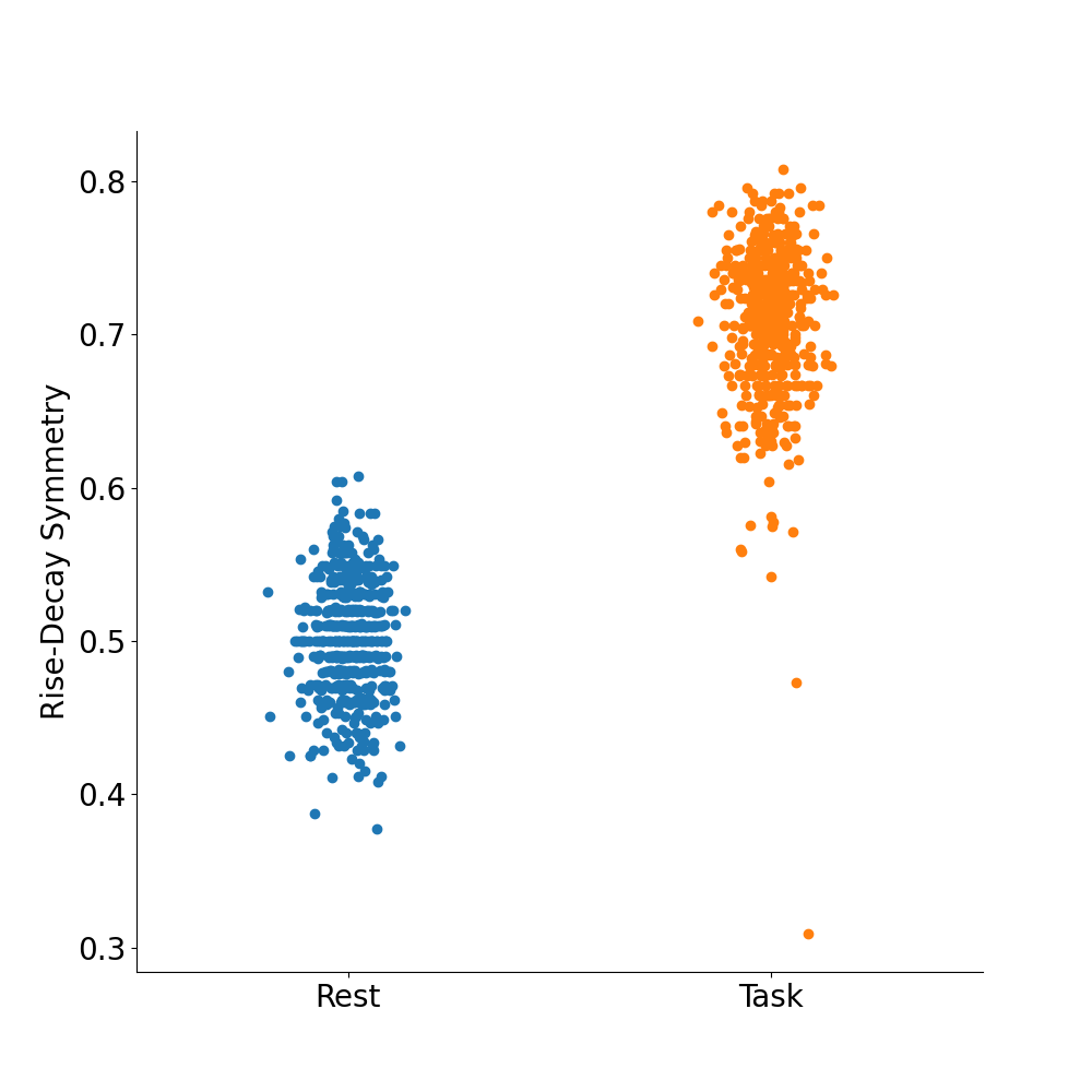
# Define rdsym values for rest and task trials
rdsym_rest = 0.5
rdsym_task = 0.75

# Simulate timeseries
sigs_rest = np.zeros((n_epochs, n_seconds*fs))
sigs_task = np.zeros((n_epochs, n_seconds*fs))

# Rest epoch
sim_components_rest = {'sim_powerlaw': dict(exponent=-2),
                       'sim_bursty_oscillation': dict(freq=10, cycle='asine',
                                                      enter_burst=0.75, rdsym=rdsym_rest)}

# Task epoch
sim_components_task = {'sim_powerlaw': dict(exponent=-2),
                       'sim_bursty_oscillation': dict(freq=10, cycle='asine',
                                                      enter_burst=0.75, rdsym=rdsym_task)}

for ep_idx in range(n_epochs):
    sigs_rest[ep_idx] = sim_combined(n_seconds, fs, components=sim_components_rest)
    sigs_task[ep_idx] = sim_combined(n_seconds, fs, components=sim_components_task)

# Compute features with default bycycle thresholds
thresholds = {
    'amp_fraction':0.,
    'amp_consistency': .5,
    'period_consistency': .5,
    'monotonicity': .8,
    'min_n_cycles': 3
}

bg_task = BycycleGroup(thresholds=thresholds)
bg_task.fit(sigs_task, fs, f_range, axis=None)

bg_rest = BycycleGroup(thresholds=thresholds)
bg_rest.fit(sigs_rest, fs, f_range, axis=None)

# Merge into a single dataframe
df_task = flatten_dfs(bg_task.df_features, ['task'] * len(bg_task), 'Epoch')
df_rest = flatten_dfs(bg_rest.df_features, ['rest'] * len(bg_rest), 'Epoch')

# Limit to bursting cycles
df_task_bursts = df_task[df_task['is_burst'] == True]
df_rest_bursts = df_rest[df_rest['is_burst'] == True]

df_bursts = pd.concat([df_task_bursts, df_rest_bursts], axis=0)

# Plot
plot_feature_categorical(df_bursts, 'time_rdsym', group_by='Epoch', ylabel='Rise-Decay Symmetry',
                         xlabel=['Rest', 'Task'])