3. Cycle-by-cycle analysis of resting state data

Simulated experiment using the cycle-by-cycle approach.

Say we ran an experiment and want to compare subjects’ resting state data for some reason. Maybe we want to study age, gender, disease state, or something. This has often been done to study differences in oscillatory power or coupling between groups of people. In this notebook, we will run through how to use bycycle to analyze resting state data.

In this example, we have 20 subjects (10 patients, 10 control), and we for some reason hypothesized that their alpha oscillations may be systematically different. For example, we think the patient group should have more top-down input that increases the synchrony in the oscillatory input (measured by its symmetry).

import numpy as np
from scipy import stats
import matplotlib.pyplot as plt
import pandas as pd

from neurodsp.sim import sim_combined
from neurodsp.filt import filter_signal
from neurodsp.plts import plot_time_series

from bycycle import BycycleGroup
from bycycle.plts import plot_burst_detect_summary, plot_feature_categorical

pd.options.display.max_columns = 10

Load simulated experiment of 10 patients and 10 controls

# Simulate experimental data
np.random.seed(0)
n_seconds = 10
fs = 1000
n_subjects = 20
sigs = np.zeros((n_subjects, int(fs * n_seconds)))

for subject_idx in range(n_subjects):

    # Manipulate the rise-decay symmetry between the two groups
    rdsym = .35 if subject_idx <= int(n_subjects/2) else 0.5

    components = {'sim_bursty_oscillation': {'freq': 10, 'enter_burst': .1, 'leave_burst': .1,
                                             'cycle': 'asine', 'rdsym': rdsym},
                  'sim_powerlaw': {'f_range': (2, None)}}

    sigs[subject_idx] = sim_combined(n_seconds, fs, components=components, component_variances=(5, 1))


# Apply lowpass filter to each signal
for idx in range(len(sigs)):
    sigs[idx] = filter_signal(sigs[idx], fs, 'lowpass', 30, n_seconds=.2, remove_edges=False)

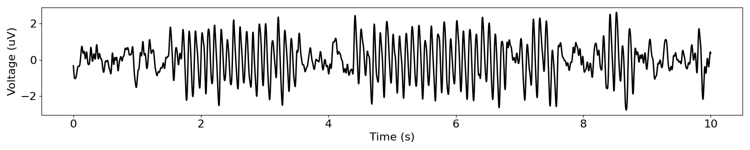
# Plot an example signal
n_signals = len(sigs)
n_seconds = len(sigs[0])/fs
times = np.arange(0, n_seconds, 1/fs)

plot_time_series(times, sigs[0], lw=2)

Compute cycle-by-cycle features

# Frequency band of interest
f_alpha = (7, 13)

# Tuned burst detection parameters
thresholds = {
    'amp_fraction': .2,
    'amp_consistency': .5,
    'period_consistency': .5,
    'monotonicity': .9,
    'min_n_cycles': 2
}

# Compute features for each signal
bg = BycycleGroup(thresholds=thresholds)
bg.fit(sigs, fs, f_alpha)

# Recompute cycles on edges of bursts with reduced thresholds
bg.recompute_edges(.01)

# Add group and subject ids to dataframes
groups = ['patient' if idx >= int(n_signals/2) else 'control' for idx in range(n_signals)]
subject_ids = [idx for idx in range(n_signals)]

for idx, group in enumerate(groups):
    bg.df_features[idx]['group'] = group
    bg.df_features[idx]['subject_id'] = subject_ids[idx]

# Concatenate the list of dataframes
df_features = pd.concat(bg.df_features)

df_features.head()

	amp_fraction	amp_consistency	period_consistency	monotonicity	period	...	sample_last_trough	sample_next_trough	is_burst	group	subject_id
0	0.234043	NaN	NaN	0.856481	153	...	89	242	False	control	0
1	0.202128	0.806234	0.385621	0.980769	59	...	242	301	False	control	0
2	0.191489	0.337052	0.627660	0.792573	94	...	301	395	False	control	0
3	0.095745	0.239360	0.699115	1.000000	79	...	395	474	False	control	0
4	0.117021	0.634007	0.699115	0.895161	113	...	474	587	False	control	0

5 rows × 26 columns

Confirm appropriateness of burst detection parameters

These burst detection parameters seem appropriate because they mostly restrict the analysis to periods of the signal that appear to be bursting. This was confirmed by looking at a few different signal segments from a few subjects.

bg[0].plot(xlim=(0, 10), figsize=(16, 3))

/Users/ryanhammonds/projects/bycycle/.env/lib/python3.11/site-packages/neurodsp/plts/style.py:69: MatplotlibDeprecationWarning: MarkerStyle(None) is deprecated since 3.6; support will be removed two minor releases later.  Use MarkerStyle('') to construct an empty MarkerStyle.
  line.set(**{style : next(values)})
/Users/ryanhammonds/projects/bycycle/.env/lib/python3.11/site-packages/neurodsp/plts/style.py:69: MatplotlibDeprecationWarning: MarkerStyle(None) is deprecated since 3.6; support will be removed two minor releases later.  Use MarkerStyle('') to construct an empty MarkerStyle.
  line.set(**{style : next(values)})
/Users/ryanhammonds/projects/bycycle/.env/lib/python3.11/site-packages/neurodsp/plts/style.py:69: MatplotlibDeprecationWarning: MarkerStyle(None) is deprecated since 3.6; support will be removed two minor releases later.  Use MarkerStyle('') to construct an empty MarkerStyle.
  line.set(**{style : next(values)})
/Users/ryanhammonds/projects/bycycle/.env/lib/python3.11/site-packages/neurodsp/plts/style.py:69: MatplotlibDeprecationWarning: MarkerStyle(None) is deprecated since 3.6; support will be removed two minor releases later.  Use MarkerStyle('') to construct an empty MarkerStyle.
  line.set(**{style : next(values)})

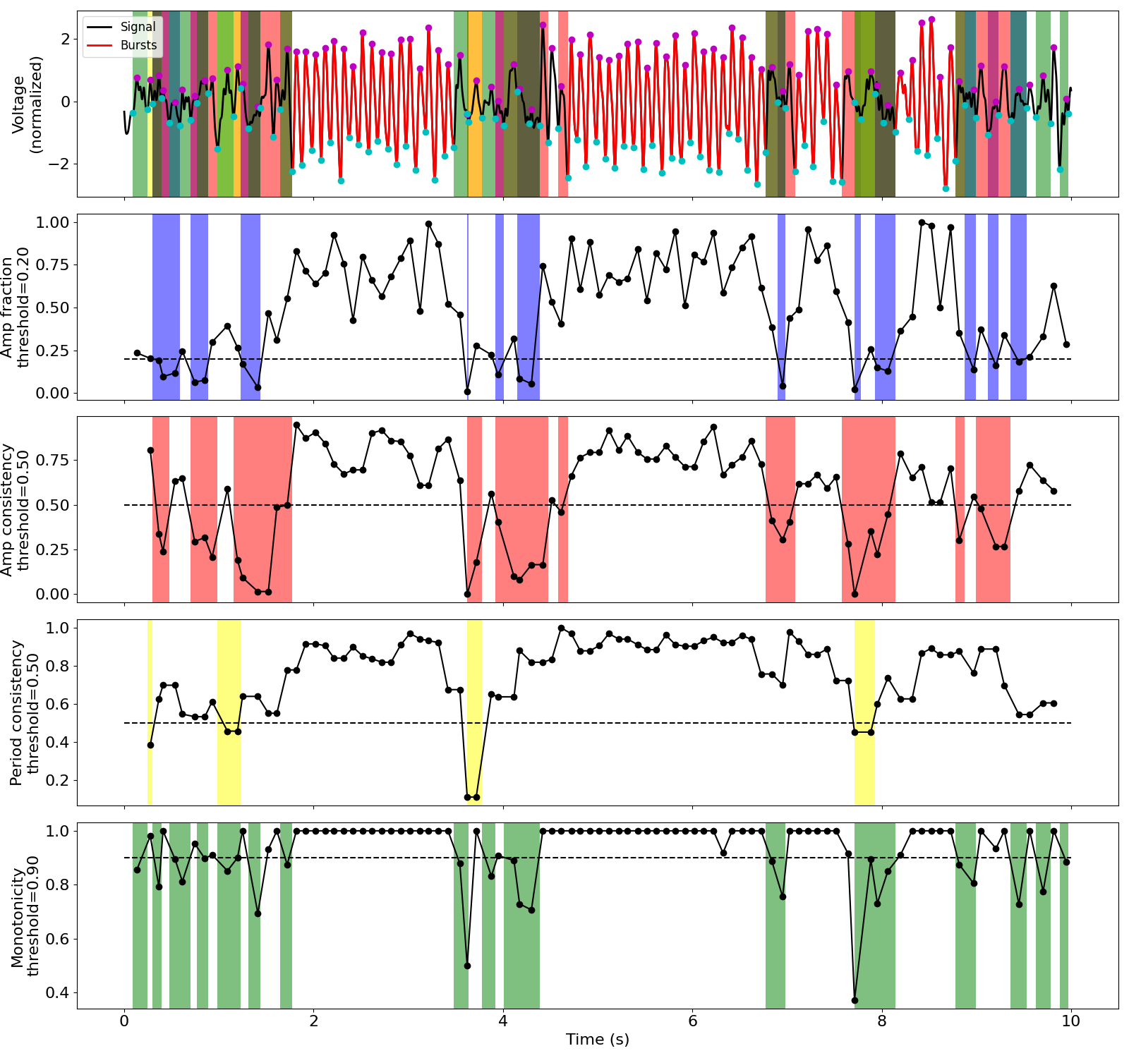
Analyze cycle-by-cycle features

Note the significant difference between the treatment and control groups for rise-decay symmetry but not the other features.

# Only consider cycles that were identified to be in bursting regimes
df_features_burst = df_features[df_features['is_burst']]

# Compute average features across subjects in a recording
features_keep = ['volt_amp', 'period', 'time_rdsym', 'time_ptsym']
df_subjects = df_features_burst.groupby(['group', 'subject_id']).mean()[features_keep].reset_index()
df_subjects.head()

	group	subject_id	volt_amp	period	time_rdsym	time_ptsym
0	control	0	3.415119	99.645833	0.398167	0.506239
1	control	1	3.663709	102.357143	0.417092	0.503348
2	control	2	3.830204	99.142857	0.392477	0.511995
3	control	3	3.555657	98.945946	0.410615	0.499541
4	control	4	4.496516	100.062500	0.406571	0.508676

fig, axes = plt.subplots(figsize=(15, 15), nrows=2, ncols=2)


plot_feature_categorical(df_subjects, 'volt_amp', group_by='group', ax=axes[0][0],
                         xlabel=['Patient', 'Control'], ylabel='Amplitude')

plot_feature_categorical(df_subjects, 'period', group_by='group', ax=axes[0][1],
                         xlabel=['Patient', 'Control'], ylabel='Period (ms)')

plot_feature_categorical(df_subjects, 'time_rdsym', group_by='group', ax=axes[1][0],
                         xlabel=['Patient', 'Control'], ylabel='Rise-Decay Symmetry')

plot_feature_categorical(df_subjects, 'time_ptsym', group_by='group', ax=axes[1][1],
                         xlabel=['Patient', 'Control'], ylabel='Peak-Trough Symmetry')

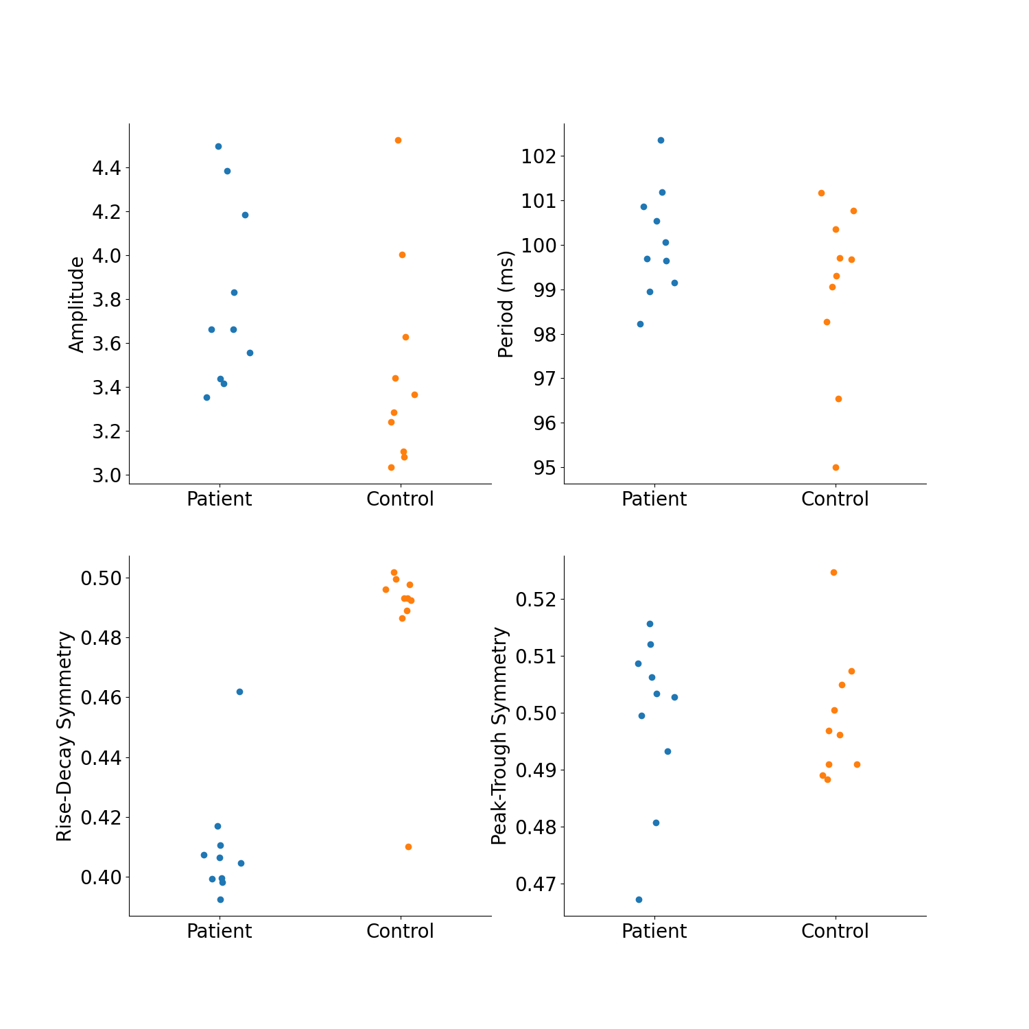
Statistical differences in cycle features

feature_names = {'volt_amp': 'Amplitude',
                 'period': 'Period (ms)',
                 'time_rdsym': 'Rise-Decay Symmetry',
                 'time_ptsym': 'Peak-Trough Symmetry'}

for feat, feat_name in feature_names.items():

    x_treatment = df_subjects[df_subjects['group'] == 'patient'][feat]
    x_control = df_subjects[df_subjects['group'] == 'control'][feat]
    ustat, pval = stats.mannwhitneyu(x_treatment, x_control)
    print('{:20s} difference between groups, U= {:3.0f}, p={:.5f}'.format(feat_name, ustat, pval))

Amplitude            difference between groups, U=  25, p=0.06402
Period (ms)          difference between groups, U=  36, p=0.30749
Rise-Decay Symmetry  difference between groups, U=  97, p=0.00044
Peak-Trough Symmetry difference between groups, U=  41, p=0.52052