3. MNE Interface Cycle Feature Distributions

Compute bycycle feature distributions using MNE objects.

Import Packages and Load Data

First let’s import the packages we need. This example depends on mne.

import numpy as np
import matplotlib.pyplot as plt

from mne.io import read_raw_fif
from mne.datasets import sample
from mne import pick_channels

from neurodsp.plts import plot_time_series
from bycycle import BycycleGroup
from bycycle.plts import plot_feature_hist

# Frequencies of interest: the alpha band
f_alpha = (8, 15)

# Get the data path for the MNE example data
raw_fname = str(sample.data_path()) + '/MEG/sample/sample_audvis_filt-0-40_raw.fif'

# Load the file of example MNE data
raw = read_raw_fif(raw_fname, preload=True, verbose=False)

# Select EEG channels from the dataset
raw = raw.pick_types(meg=False, eeg=True, eog=False, exclude='bads')

# Grab the sampling rate from the data
fs = raw.info['sfreq']

# filter to alpha
raw = raw.filter(l_freq=None, h_freq=20.)

# Settings for exploring example channels of data
chs = ['EEG 042', 'EEG 043', 'EEG 044']
t_start = 20000
t_stop = int(t_start + (10 * fs))

# Extract an example channels to explore
sigs, times = raw.get_data(pick_channels(raw.ch_names, chs),
                           start=t_start, stop=t_stop, return_times=True)

Removing projector <Projection | PCA-v1, active : False, n_channels : 102>
Removing projector <Projection | PCA-v2, active : False, n_channels : 102>
Removing projector <Projection | PCA-v3, active : False, n_channels : 102>
Filtering raw data in 1 contiguous segment
Setting up low-pass filter at 20 Hz

FIR filter parameters
---------------------
Designing a one-pass, zero-phase, non-causal lowpass filter:
- Windowed time-domain design (firwin) method
- Hamming window with 0.0194 passband ripple and 53 dB stopband attenuation
- Upper passband edge: 20.00 Hz
- Upper transition bandwidth: 5.00 Hz (-6 dB cutoff frequency: 22.50 Hz)
- Filter length: 101 samples (0.673 sec)

[Parallel(n_jobs=1)]: Using backend SequentialBackend with 1 concurrent workers.
[Parallel(n_jobs=1)]: Done   1 out of   1 | elapsed:    0.0s remaining:    0.0s
[Parallel(n_jobs=1)]: Done   2 out of   2 | elapsed:    0.0s remaining:    0.0s
[Parallel(n_jobs=1)]: Done   3 out of   3 | elapsed:    0.0s remaining:    0.0s
[Parallel(n_jobs=1)]: Done   4 out of   4 | elapsed:    0.0s remaining:    0.0s
[Parallel(n_jobs=1)]: Done  59 out of  59 | elapsed:    0.0s finished

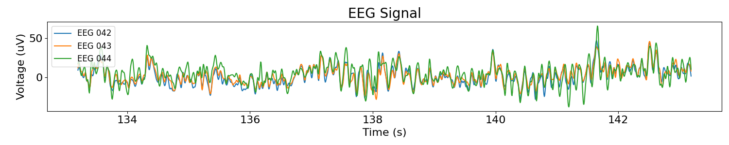
Plot time series for each recording

Now let’s see how each signal looks in time. This looks like standard EEG data.

# Plot the signal
plot_time_series(times, [sig * 1e6 for sig in sigs], labels=chs, title='EEG Signal')

Compute cycle-by-cycle features

Here we use the BycycleGroup class to compute the cycle-by- cycle features of the three signals.

# Set parameters for defining oscillatory bursts
thresholds = {
    'amp_fraction_threshold': 0.3,
    'amp_consistency_threshold': 0.4,
    'period_consistency_threshold': 0.5,
    'monotonicity_threshold': 0.8,
    'min_n_cycles': 3
}

# Create a dictionary of cycle feature dataframes, corresponding to each channel
bg = BycycleGroup(thresholds=thresholds, center_extrema='trough')
bg.fit(sigs, fs, f_alpha, axis=0)

dfs = {ch: df for df, ch in zip(bg.df_features, chs)}

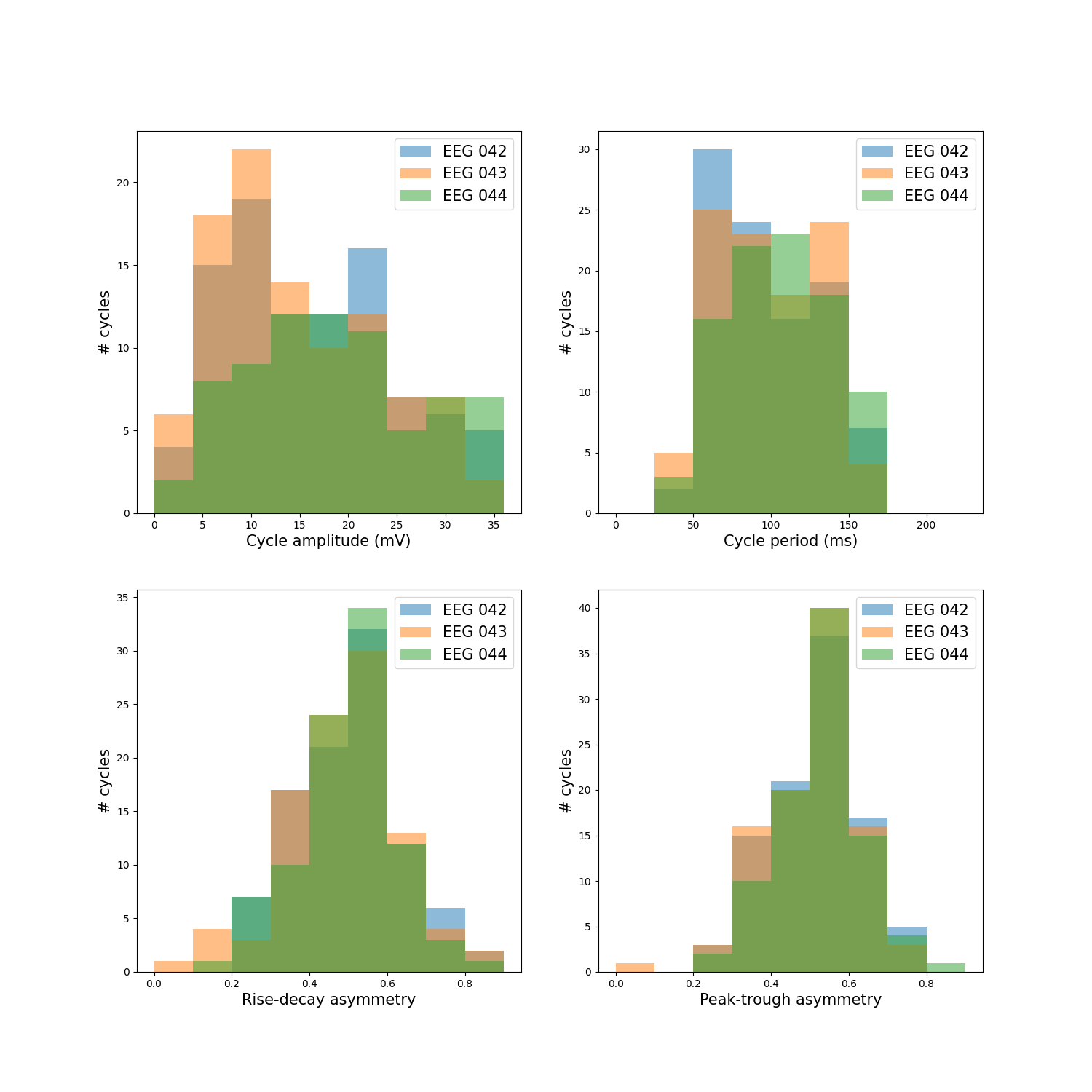
Plot feature distributions

As it turns out, none of the channels in the mne example audio and visual task has waveform asymmetry. These data were collected from a healthy person while they listened to beeps or saw gratings on a screen so this is not unexpected.

fig, axes = plt.subplots(figsize=(15, 15), nrows=2, ncols=2)

for ch, df in dfs.items():

    # Rescale amplitude and period features
    df['volt_amp'] = df['volt_amp'] * 1e6
    df['period'] = df['period'] / fs * 1000

    # Plot feature histograms
    plot_feature_hist(df, 'volt_amp', only_bursts=False, ax=axes[0][0], label=ch,
                      xlabel='Cycle amplitude (mV)', bins=np.arange(0, 40, 4))

    plot_feature_hist(df, 'period', only_bursts=False, ax=axes[0][1], label=ch,
                      xlabel='Cycle period (ms)', bins=np.arange(0, 250, 25))

    plot_feature_hist(df, 'time_rdsym', only_bursts=False, ax=axes[1][0], label=ch,
                      xlabel='Rise-decay asymmetry', bins=np.arange(0, 1, .1))

    plot_feature_hist(df, 'time_ptsym', only_bursts=False, ax=axes[1][1], label=ch,
                      xlabel='Peak-trough asymmetry', bins=np.arange(0, 1, .1))