1. Theta oscillation cycle feature distributions

Compute and compare the distributions of bycycle features for two recordings.

import numpy as np
import matplotlib.pyplot as plt

from neurodsp.filt import filter_signal
from neurodsp.plts import plot_time_series

from bycycle import BycycleGroup
from bycycle.plts.features import plot_feature_hist
from bycycle.utils.download import load_bycycle_data

Load and preprocess data

# Load data
ca1_raw = load_bycycle_data('ca1.npy', folder='data')
ec3_raw = load_bycycle_data('ec3.npy', folder='data')
fs = 1250
f_theta = (4, 10)

# Apply a lowpass filter at 25Hz
fc = 25
filter_seconds = .5

ca1 = filter_signal(ca1_raw, fs, 'lowpass', fc, n_seconds=filter_seconds,
                    remove_edges=False)
ec3 = filter_signal(ec3_raw, fs, 'lowpass', fc, n_seconds=filter_seconds,
                    remove_edges=False)

Compute cycle-by-cycle features

# Set parameters for defining oscillatory bursts
thresholds = {
    'amp_fraction_threshold': 0,
    'amp_consistency_threshold': .6,
    'period_consistency_threshold': .75,
    'monotonicity_threshold': .8,
    'min_n_cycles': 3
}

# Cycle-by-cycle analysis
sigs = np.array([ca1, ec3])

bg = BycycleGroup(thresholds=thresholds, center_extrema='trough', return_samples=False)
bg.fit(sigs, fs, f_theta)

df_ca1, df_ec3 = bg.df_features

# Limit analysis only to oscillatory bursts
df_ca1_cycles = df_ca1[df_ca1['is_burst']]
df_ec3_cycles = df_ec3[df_ec3['is_burst']]

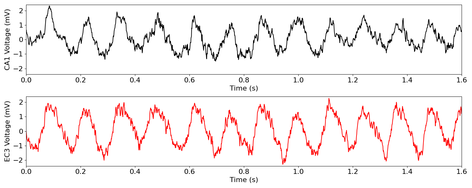
Plot time series for each recording

# Choose samples to plot
samplims = (10000, 12000)
ca1_plt = ca1_raw[samplims[0]:samplims[1]]
ec3_plt = ec3_raw[samplims[0]:samplims[1]]
times = np.arange(0, len(ca1_plt)/fs, 1/fs)

fig, axes = plt.subplots(figsize=(15, 6), nrows=2)

plot_time_series(times, ca1_plt, ax=axes[0], xlim=(0, 1.6), ylim=(-2.4, 2.4),
                 xlabel="Time (s)", ylabel="CA1 Voltage (mV)")

plot_time_series(times, ec3_plt, ax=axes[1], colors='r', xlim=(0, 1.6),
                 ylim=(-2.4, 2.4), xlabel="Time (s)", ylabel="EC3 Voltage (mV)")

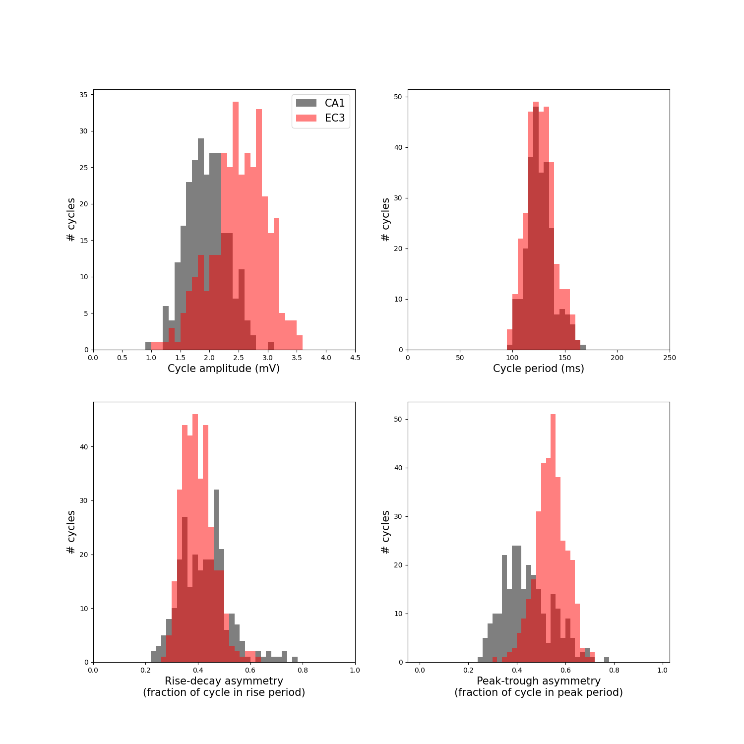
Plot feature distributions

fig, axes = plt.subplots(figsize=(15, 15), nrows=2, ncols=2)

# Plot cycle amplitude
cycles_ca1 = df_ca1_cycles['volt_amp']
cycles_ec3 = df_ec3_cycles['volt_amp']

plot_feature_hist(cycles_ca1, 'volt_amp', ax=axes[0][0], xlabel='Cycle amplitude (mV)',
                  xlim=(0, 4.5), color='k', bins=np.arange(0, 8, .1))

plot_feature_hist(cycles_ec3, 'volt_amp', ax=axes[0][0], xlabel='Cycle amplitude (mV)',
                  xlim=(0, 4.5), color='r', bins=np.arange(0, 8, .1))

axes[0][0].legend(['CA1', 'EC3'], fontsize=15)

# Plot cycle period
periods_ca1 = df_ca1_cycles['period'] / fs * 1000
periods_ec3 = df_ec3_cycles['period'] / fs * 1000

plot_feature_hist(periods_ca1, 'period', ax=axes[0][1], xlabel='Cycle period (ms)',
                  xlim=(0, 250), color='k', bins=np.arange(0, 250, 5))

plot_feature_hist(periods_ec3, 'volt_amp', ax=axes[0][1], xlabel='Cycle period (ms)',
                  xlim=(0, 250), color='r', bins=np.arange(0, 250, 5))

# Plot rise/decay symmetry
plot_feature_hist(df_ca1_cycles, 'time_rdsym', ax=axes[1][0], xlim=(0, 1), color='k',
                  xlabel='Rise-decay asymmetry\n(fraction of cycle in rise period)',
                  bins=np.arange(0, 1, .02))

plot_feature_hist(df_ec3_cycles, 'time_rdsym', ax=axes[1][0], xlim=(0, 1), color='r',
                  xlabel='Rise-decay asymmetry\n(fraction of cycle in rise period)',
                  bins=np.arange(0, 1, .02))

# Plot peak/trough symmetry
plot_feature_hist(df_ca1_cycles, 'time_ptsym', ax=axes[1][1], color='k',
                  xlabel='Peak-trough asymmetry\n(fraction of cycle in peak period)',
                  bins=np.arange(0, 1, .02))

plot_feature_hist(df_ec3_cycles, 'time_ptsym', ax=axes[1][1], color='r',
                  xlabel='Peak-trough asymmetry\n(fraction of cycle in peak period)',
                  bins=np.arange(0, 1, .02))