bycycle.plts.plot_cyclepoints_array
- bycycle.plts.plot_cyclepoints_array(sig, fs, peaks=None, troughs=None, rises=None, decays=None, plot_sig=True, xlim=None, ax=None, **kwargs)[source]
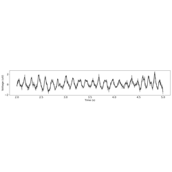
Plot extrema and/or zero-crossings from arrays.
- Parameters:
- sig1d array
Time series to plot.
- fsfloat
Sampling rate, in Hz.
- peaks1d array, optional
Peak signal indices from
find_extrema().- troughs1d array, optional
Trough signal indices from
find_extrema().- rises1d array, optional
Zero-crossing rise indices from
find_zerox().- decays1d array, optional
Zero-crossing decay indices from
find_zerox().- plot_sigbool, optional, default: True
Whether to also plot the raw signal.
- xlimtuple of (float, float), optional
Start and stop times.
- axmatplotlib.Axes, optional, default: None
Figure axes upon which to plot.
- **kwargs
Keyword arguments to pass into plot_time_series.
Notes
Default keyword arguments include:
figsize: tuple of (float, float), default: (15, 3)xlabel: str, default: ‘Time (s)’ylabel: str, default: ‘Voltage (uV)colors: list, default: [‘k’, ‘b’, ‘r’, ‘g’, ‘m’]
Examples
Plot cyclepoints using arrays from
find_extrema()andfind_zerox():>>> from bycycle.cyclepoints import find_extrema, find_zerox >>> from neurodsp.sim import sim_bursty_oscillation >>> fs = 500 >>> sig = sim_bursty_oscillation(10, fs, freq=10) >>> peaks, troughs = find_extrema(sig, fs, f_range=(8, 12), boundary=0) >>> rises, decays = find_zerox(sig, peaks, troughs) >>> plot_cyclepoints_array(sig, fs, peaks=peaks, troughs=troughs, rises=rises, decays=decays)